Goal
In this blog post, I am going to introduce spectral clustering and want to write a tutorial on a simple version of the spectral clustering algorithm for clustering data points with visual demonstrations.
Introduction -- What is clustering?
When a data set with a large amount of data points is given, it is sometimes hard to categorize all the data points in meaningful groups that we usually called such a separation step as clustering. Spectral clustering is one of the most important analysis tools for identifying various parts in one complex-structure data set. Before discussing how to use spectral clustering for group identification within data sets, we are going to show few examples to understand the meaning of separating data sets into groups by using the k-means -- another common method to separate data sets when data sets distributed as two natural "blobs."
Packages
First of all, we need to import the packages we are going to use throughout the tutorial.
# common package for array analysis
import numpy as np
# generate data set
from sklearn import datasets
# plot graphs
from matplotlib import pyplot as plt
# k-means for separation of data sets with two natural "blobs"
from sklearn.cluster import KMeans
# compute the distance between two data points of an array by forming a matrix
from sklearn.metrics.pairwise import pairwise_distances
# minimize scalar functions
from scipy.optimize import minimize
Clustering Examples By K-Means
Now, we are ready to generate a random data set and show its distributions of the data points by creating a scatterplot.
# set the size of the data set
n = 200
# control the randomness for each time running this cell
np.random.seed(1111)
# generate a date set of size n in a matrix with the Euclidean coordinates of the data
# points forming as two blobs and a data set of size n with integer labels of each blob
X, y = datasets.make_blobs(n_samples = n, shuffle = True, random_state = None, centers = 2, cluster_std = 2.0)
# plot a scatterplot based on the Euclidean coordinates of the data points
plt.scatter(X[:,0], X[:,1])
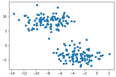
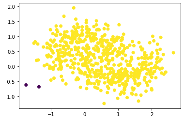
Based on the above graph showing the data set we just created, it is easy to notice that the data set mainly forms two clusters, which is caused by using datasets.make_blobs. Then, we want to use the k-means to separate those two clusters in different colors since k-means is good at separating circular-ish blobs.
# compute k-means clustering with two clusters
km = KMeans(n_clusters = 2)
# fit the data points in k-means
km.fit(X)
# plot a scatterplot based on the Euclidean coordinates of the
# data points with a group color, predicting by the k-means
plt.scatter(X[:,0], X[:,1], c = km.predict(X))
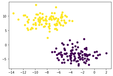
It can be seen that the data set is clearly categorized into two groups, and each point is in either yellow or purple by the k-means. However, the k-means algorithm might not be always good at clustering when the data set is in other shapes. Let's see an example below.
# set the size of the data set
n = 200
# control the randomness for each time running this cell
np.random.seed(1234)
# generate a date set of size n with data points forming as two
# moons and a data set of size n with integer labels of each moon
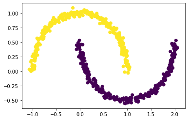
X, y = datasets.make_moons(n_samples = n, shuffle = True, noise = 0.05, random_state = None)
# plot a scatterplot based on the Euclidean coordinates of the data points
plt.scatter(X[:,0], X[:,1])
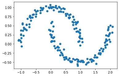
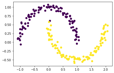
Obviously, there are still two clusters in the data set. The data set no longer looks like two blobs. Instead, the data set looks like two crescents. Similar to what we did in the previous steps, we are going to use k-means again to predict the clusters in this data set.
# compute k-means clustering with two clusters
km = KMeans(n_clusters = 2)
# fit the data points in k-means
km.fit(X)
# plot a scatterplot based on the Euclidean coordinates of the
# data points with a group color, predicting by the k-means
plt.scatter(X[:,0], X[:,1], c = km.predict(X))
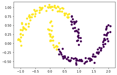
By using the k-means here, we found out that the k-means did not completely separate the two crescents in the data set since each crescent contains both yellow and purple data points. This is because k-means is good at separating circular clusters by design.
So, we are going to learn how to use spectral clustering to correctly cluster these two crescents in the following several parts.
Spectral Clustering
Part A -- How to create a similarity matrix?
Firstly, we need to construct the similarity matrix $$\mathbf{A}$$ with the following requirements:
-
$$\mathbf{A}$$ is a matrix, forming by 2d
np.ndarray, withnrows andncolumns wherenis the number of data points. -
Each entry in $$\mathbf{A}$$ is calculated by finding whether the distance between two points in the matrix
Xis withinepsilon. We will considerepsilonto be0.4for this part. -
The diagonal entries in $$\mathbf{A}$$, which are the entries where the row number equals the column number, should all be equal to
0.
Recall that in the Introduction, we defined the following variables:
-
n: the size of the data set, which is200 -
$$\mathbf{X}$$: a matrix containing the Euclidean coordinates of the data points
-
$$\mathbf{y}$$: a vector containing the labels of each point
In order to calculate the distance between two data points, we will use pairwise_distances from the sklearn package, and this will generate a matrix containing value in each entry as the distance between two data points in the matrix $$\mathbf{X}$$. For instance, the value in the first row and second column of the output matrix represents the distance between the first point and the second point in the matrix $$\mathbf{X}$$. Comparing to epsilonand then multiplying by 1.0, we will get a matrix consisting of 0. and 1.. Lastly, we will use np.fill_diagonal() to make the diagonal entries of a matrix to become a certain value. For the similarity matrix here, we will make its diagonal entries be 0.
# set the value of the epsilon that decides the distance between two points
epsilon = 0.4

# find the matrix A where the entry is 1 if the distance between two points in X is within epsilon
# and the entry is 0 if the distance between two points in X is greater than epsilon
A = (pairwise_distances(X) <= epsilon)*1.0

# reset the diagonal entries of the matrix A to be 0
np.fill_diagonal(A, 0)

# show the output A
A
array([[0., 0., 0., ..., 0., 0., 0.],
       [0., 0., 0., ..., 0., 0., 0.],
       [0., 0., 0., ..., 0., 1., 0.],
       ...,
       [0., 0., 0., ..., 0., 1., 1.],
       [0., 0., 1., ..., 1., 0., 1.],
       [0., 0., 0., ..., 1., 1., 0.]])
Part B -- How to calculate the binary norm cut objective with the similarity matrix?
From Part A, we have the similarity matrix $$\mathbf{A}$$ showing whether each point is within distance, epsilon, to other points. Recall that the cluster membership $$\mathbf{y}$$ contains values of 0 and 1 as the labels of the data points in $$\mathbf{X}$$. For this part, we want to figure out how to cluster the data points in $$\mathbf{X}$$ by using the binary norm cut objective of the similarity matrix $$\mathbf{A}$$:
$$N_{\mathbf{A}}(C_0, C_1)\equiv \mathbf{cut}(C_0, C_1)\left(\frac{1}{\mathbf{vol}(C_0)} + \frac{1}{\mathbf{vol}(C_1)}\right);.$$
where
- $$\mathbf{cut}(C_0, C_1) \equiv \sum_{i \in C_0, j \in C_1} a_{ij}$$ is the cut of the clusters $$C_0$$ and $$C_1$$, where $$C_0$$ and $$C_1$$ are the two clusters of the data points in $$\mathbf{X}$$.
- $$\mathbf{vol}(C_0) \equiv \sum_{i \in C_0}d_i$$, where $$d_i = \sum_{j = 1}^n a_{ij}$$ is the degree of row $$i$$ calculated by the $$i$$th row-sum of the similarity matrix $$\mathbf{A}$$.
Based on the binary norm cut objective, we may know that if $$N_{\mathbf{A}}(C_0, C_1)$$ is small, a pair of clusters $$C_0$$ and $$C_1$$ is usually considered to be a "good" partition of the data. Hence, the smaller the value of $$N_{\mathbf{A}}(C_0, C_1)$$ is, the better partition of the pair, $$C_0$$ and $$C_1$$, is.
Let's consider $$\mathbf{cut}$$ and $$\mathbf{vol}$$ separately to understand the binary norm cut objective better.
B.1 The Cut Term
The cut term $$\mathbf{cut}(C_0, C_1)$$ calculates the sum of all the entries where the two data points are in different clusters in matrix $$\mathbf{A}$$. Thus, it represents the number of nonzero entries in $$\mathbf{A}$$ that relate points in cluster $$C_0$$ to points in cluster $$C_1$$. We also know that the value 0. in $$\mathbf{A}$$ represents the distance between two points are greater than epsilon. Hence, the smaller the cut term is, the further the distance between the points in $$C_0$$ and the points in $$C_1$$ is.
Based on the definition of the cut term above, we are going to define a cut(A, y) function that takes a similarity matrix $$\mathbf{A}$$ and a vector $$\mathbf{y}$$ as parameters and return the value of the cut term below.
def cut(A, y):
    """
    Calculate the cut term by adding all the entries in the input
    similarity matrix A when two data points are
    not in the same cluster based on the input label vector y.

    Parameter
    ----------
    A: the input similarity matrix consisting of values 0. and 1.
    y: the input vector represents the labels of the data points

    Return
    ----------
    cut: a floating number represents the sum of all the entries where two
    points are in different clusters, found by vector y, in matrix A
    """

    # initialize cut
    cut = 0

    # use a nested for loop based on y to loop over each row and column
    # of the similarity matrix A
    for i in range(len(y)):
        for j in range(len(y)):
            if y[i] != y[j]: # if two data points are not in the same clusters
                cut = cut + A[i, j] # add the value of that entry in A to cut

    return cut
By using the similarity matrix $$\mathbf{A}$$ and the vector $$\mathbf{y}$$ as the true labels defined before, let's see what the cut objective is for our data set defined at the beginning.
cut(A, y) # cut term of true labels y
26.0
Thus, we have the cut objective for the true labels $$\mathbf{y}$$ to be 26.0. Then, we want to also generate a fake random labels called $$\mathbf{rand_vec}$$, which is a random vector of random labels of the same length n with each label as either 0 or 1, for comparison and we also check the cut objectives for $$\mathbf{rand_vec}$$.
# control the randomness for each time running this cell
np.random.seed(1234)
# generate a random vector of length n with 0 and 1 as labels
rand_vec = np.random.randint(0, 2, n)
# cut term of fake labels rand_vec
cut(A, rand_vec)
2308.0
Thus, we have that the cut objective for the fake random labels $$\mathbf{rand_vec}$$ is 2308.0, which is much larger than the one for the true labels $$\mathbf{y}$$ above, which means that the points in $$C_0$$ and the points in $$C_1$$ are much closer produced by the fake random labels $$\mathbf{rand_vec}$$.
B.2 The Volume Term
The second factor in the binary norm cut objective equation we are going to investigate is the volumn term, $$\mathbf{vol}(C_0)$$ and $$\mathbf{vol}(C_1)$$. The larger the volumn term of a cluster is, the bigger the cluster is. Recall that a certain row in a similiarity matrix $$\mathbf{A}$$ represents the whether the first data point is far away from the rest of the data points.
In this part, we need to first find the rows in $$\mathbf{A}$$ correspond to a certain label and sum all these rows in $$\mathbf{A}$$ in order to calculate the size of each cluster -- the volume term of each cluster. We want to write a function called vols(A, y) that takes a similarity matrix $$\mathbf{A}$$ and a vector $$\mathbf{y}$$ as parameters and return the value of the volume term for each $$C_0$$ and $$C_1$$ in a tuple below.
def vols(A, y):
    """
    Calculate the volume term for each cluster by adding all the entries
    in the input similarity matrix A for the data points in the same
    cluster based on the input label vector y.

    Parameter
    ----------
    A: the input similarity matrix consisting of values 0. and 1.
    y: the input vector represents the labels of the data points

    Return
    ----------
    v0, v1: a tuple consisting two floating numbers where each floating number
    represents the volume term of a cluster
    """

    # find the sum of the rows in A where the value in true labels y equals 0
    v0 = np.sum(A[y == 0])

    # find the sum of the rows in A where the value in true labels y equals 1
    v1 = np.sum(A[y == 1])
    return v0, v1
Let's check for the volume terms, $$\mathbf{vol}(C_0)$$ and $$\mathbf{vol}(C_1)$$, by using the true labels $$\mathbf{y}$$.
# volume terms of true labels y
v0, v1 = vols(A, y)
v0, v1
(2299.0, 2217.0)
Thus, we have that $$\mathbf{vol}(C_0)$$ is 2299.0, which is larger than $$\mathbf{vol}(C_1)$$ with a value of 2217.0 by using the true labels $$\mathbf{y}$$.
Let's check for the volume terms, $$\mathbf{vol}(C_0)$$ and $$\mathbf{vol}(C_1)$$, by using the fake labels $$\mathbf{rand_vec}$$.
# volume terms of fake labels rand_vec
v0_fake, v1_fake = vols(A, rand_vec)
v0_fake, v1_fake
(2336.0, 2180.0)
Thus, we have that $$\mathbf{vol}(C_0)$$ is 2336.0, which is larger than $$\mathbf{vol}(C_1)$$ with a value of 2180.0 by using the fake labels $$\mathbf{rand_vec}$$.
After defining the above two functions in this part, we want to write a function called normcut(A, y) to compute the binary normalized cut objective of a similarity matrix $$\mathbf{A}$$ with clustering vector $$\mathbf{y}$$.
def normcut(A, y):
    """
    Calculate the binary norm cut objective by using the cut(A, y) function
    and the vols(A, y) function based on the binary norm cut objective equation.

    Parameter
    ----------
    A: the input similarity matrix consisting of values 0. and 1.
    y: the input vector represents the labels of the data points

    Return
    ----------
    binary: a floating number represents the binary norm cut objective
    """

    # define binary by using the cut(A, y) function and the vols(A, y) function
    # based on the binary normalized cut objective equation
    binary = cut(A, y)*(1/vols(A, y)[0] + 1/vols(A, y)[1])
    return binary
Now, let's compare the normcut objective using both the true labels $$\mathbf{y}$$ and the fake labels $$\mathbf{rand_vec}$$ defined above by using our normcut(A, y) function.
# normcut objective of true labels y
normcut(A, y)
0.02303682466323045
# normcut objective of fake labels rand_vec
normcut(A, rand_vec)
2.046729294960412
Thus, the normcut objective by using the true labels $$\mathbf{y}$$ is about 0.02304, and one by using the fake labels $$\mathbf{rand_vec}$$ is about 2.04673. Comparing these two normcut objectives, we may conclude that the normcut objective of the fake labels is much higher than the true labels. Considering both the cut term and the volume term above, we may realize that the large cut term might cause the normcut objective of the fake labels to be large. Hence, we found out that the clusters have a better partition with the true labels than the fake labels.
Overall, the binary normcut objective should have clusters $$C_0$$ and $$C_1$$ such that:
- The clusters, $$C_0$$ and $$C_1$$, stay far away from each other to keep as few entries of $$\mathbf{A}$$ that join both clusters as possible.
- Neither the clusters, $$C_0$$ and $$C_1$$, are too small.
Part C -- How to prepare for the best clustering?
Though we might be able to find a cluster vector $$\mathbf{y}$$ such that we may get a very small normcut(A,y) which is good for clustering, the process of finding such a cluster vector to reach the best clustering is very hard. Hence, we are going to define a new vector $$\mathbf{z} \in \mathbb{R}^n$$ such that:
$$ z_i = \begin{cases} \frac{1}{\mathbf{vol}(C_0)} &\quad \text{if } y_i = 0 \ -\frac{1}{\mathbf{vol}(C_1)} &\quad \text{if } y_i = 1 \ \end{cases} $$
Then, we have:
$$\mathbf{N}_{\mathbf{A}}(C_0, C_1) = 2\frac{\mathbf{z}^T (\mathbf{D} - \mathbf{A})\mathbf{z}}{\mathbf{z}^T\mathbf{D}\mathbf{z}};,$$
by linear algebra, where $$\mathbf{D}$$ is the diagonal matrix with nonzero entries $$d_{ii} = d_i$$, and $$d_i = \sum_{j = 1}^n a_i$$ is the degree of row $$i$$.
For this part, we are going to define a function called transform(A, y) that takes a similarity matrix $$\mathbf{A}$$ and a vector $$\mathbf{y}$$ as parameters and return $$\mathbf{z}$$.
def transform(A, y):
    """
    Create the z vector for optimal clustering based on the above zi formula.
    Specifically speaking, z vector should be constructed by making the
    entries with label 0 in y to be 1/v0, where v0 is the volume term of the
    cluster 0, and making the entries with label 1 in y to be 1/v1, where v1
    is the volume term of the cluster 1.

    Parameter
    ----------
    A: the input similarity matrix consisting of values 0. and 1.
    y: the input vector represents the labels of the data points

    Return
    ----------
    z: a numpy array represents the new vector for optimal clustering
    """

    # use the defined vols(A, y) function to calculate v0 and v1
    v0, v1 = vols(A, y)

    # find the z_c0 and z_c1 based on the formula about the new vector z above
    z_c0 = 1/v0
    z_c1 = -1/v1

    # make the entries in y with label 0 to have a value of z_c0
    # and make the entries in y with label 1 to have a value of z_c1
    z = (1 - y)*z_c0 + y*z_c1

    return z
By using the transform(A, y) function, we want to check for the difference between the matrix product and the normcut objective from the above equation. Since the computer arithmetic might not consider the equation above to be exact, we need to use np.isclose(a, b) to check whether a is "close" to b.
# get z by the transform(A, y) function
z = transform(A, y)
# find the diagonal matrix with nonzero entries of the row sum in A
D = np.diag(A.sum(axis = 1))
# check for difference
np.isclose(normcut(A, y), 2*z.T@(D - A)@z/(z.T@D@z))
True
Since the output is True, it represents that the left hand side of the equation has a difference less than the smallest amount that the computer is able to quantify from the right hand side of the equation, which we can treat this result as both sides of the equations to be equal.
By using the similar step, we also want to check for the identity $$\mathbf{z}^T\mathbf{D}\mathbb{1} = 0$$.
np.isclose(z.T@D@np.ones(n), 0) # check for difference
True
Such an output shows that the number of the positive entries is similar to the number of the negative entries in $$\mathbf{z}$$.
Part D -- How to minimize normcut objective?
We might find out that the problem of minimizing the normcut objective is mathematically related to the problem of minimizing the function
$$ R_\mathbf{A}(\mathbf{z})\equiv \frac{\mathbf{z}^T (\mathbf{D} - \mathbf{A})\mathbf{z}}{\mathbf{z}^T\mathbf{D}\mathbf{z}} $$
subject to the condition $$\mathbf{z}^T\mathbf{D}\mathbb{1} = 0$$. In order to get the orthogonal complement of $$\mathbf{z}$$ relative to $$\mathbf{D}\mathbf{1}$$ to substitute it into the equation, we may define an orth_obj function below.
def orth(u, v):
    return (u @ v) / (v @ v) * v

e = np.ones(n)

d = D @ e

def orth_obj(z):
    z_o = z - orth(z, d)
    return (z_o @ (D - A) @ z_o)/(z_o @ D @ z_o)
Next, we want to use the minimize function from scipy.optimize to minimize the function orth_obj with respect to $$\mathbf{z}$$ as $$\mathbf{z_}$$ for optimization.
# use the minimize function for minimizing orth_obj with respect to z as z_
# np.random.rand(n) is used for better minimization
z_ = minimize(orth_obj, np.random.rand(n))
Part E -- Are we able to create a perfect spectral clustering?
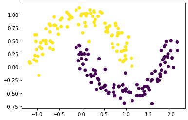
In Part C, we know that $$\mathbf{z}$$ contains value in different signs determined by the cluster labels. Similarly, we can know the information of the cluster label of data point i by checking for the sign of $$\mathbf{z_min}$$. After knowing the cluster labels for all the data points in $$\mathbf{X}$$, we are able to plot the original data by using one color for points such that z_min[i] < 0 and another color for points such that z_min[i] >= 0 for clustering.
# find the z_min by using the z_ in Part D to know the cluster membership by z_.x
z_min = z_.x
# plot a scatterplot to show the spectral clustering based on the sign of z_min
plt.scatter(X[:, 0], X[:, 1], c = z_min < 0)

Great! The data points are successfully clustered into two crescents with different colors!
Part F -- Is there a more efficient method?
However, there is actually a faster way by using eigenvalues and eigenvectors to solve the problem from Part E than explicitly optimizing the orthogonal objective.
The Rayleigh-Ritz Theorem states that the minimizing $$\mathbf{z}$$ must be the solution with smallest eigenvalue of the generalized eigenvalue problem
$$ (\mathbf{D} - \mathbf{A}) \mathbf{z} = \lambda \mathbf{D}\mathbf{z};, \quad \mathbf{z}^T\mathbf{D}\mathbb{1} = 0$$
which is equivalent to the standard eigenvalue problem
$$ \mathbf{D}^{-1}(\mathbf{D} - \mathbf{A}) \mathbf{z} = \lambda \mathbf{z};, \quad \mathbf{z}^T\mathbb{1} = 0;.$$
Since $$\mathbb{1}$$ is the eigenvector with smallest eigenvalue of the matrix $$\mathbf{D}^{-1}(\mathbf{D} - \mathbf{A})$$, we are going to figure out the vector $$\mathbf{z}$$ that we want must be the eigenvector with the second-smallest eigenvalue.
So, we need to construct the (normalized) Laplacian matrix of the similarity matrix $$\mathbf{A}$$
$$\mathbf{L} = \mathbf{D}^{-1}(\mathbf{D} - \mathbf{A})$$
to find the eigenvector $$\mathbf{z_eig}$$ corresponding to its second-smallest eigenvalue.
# construct the Laplacian matrix
L = np.linalg.inv(D)@(D - A)
# get the eigenvalues and eigenvectors from L
eig_val, eig_vec = np.linalg.eig(L)

# argsort the eigenvalues and the eigenvectors from
# the smallest eigenvalue to the largest eigenvalue
ix = eig_val.argsort()
eig_val, eig_vec = eig_val[ix], eig_vec[:, ix]

# find the eigenvector of the second-smallest eigenvalue
z_eig = eig_vec[:, 1]
Now, let's plot the data again by using the $$\mathbf{z_eig}$$ we found. Similarly, we can use the sign of $$\mathbf{z_eig}$$ to decide the cluster label.
# plot a scatterplot to show the spectral clustering based on the sign of z_eig
plt.scatter(X[:, 0], X[:, 1], c = z_eig > 0)

Hence, we found out that the data set is also clearly separated into two groups by using $$\mathbf{z_eig}$$!
Part G -- How to write the spectral clustering function?
From the several parts above, we found out that the method of finding the $$\mathbf{z_eig}$$ by using eigenvalues and eigenvectors is very efficient. Thus, we are going to summarize the several parts above to define a function called spectral_clustering(X, epsilon) by taking $$\mathbf{X}$$ and the distance threshold epsilon as input parameters and return an array of binary labels of 0. and 1..
def spectral_clustering(X, epsilon):
    """
    Generate an array of binary labels of 0 and 1 through spectral clustering.
    The function will first construct the similarity matrix A with values 0,
    if the distance between two data points is greater or equal than epsilon,
    and 1, if the distance between two data points is smaller than epsilon,
    where each entry shows whether two data points are close to each other.
    Then, the function will find the eigenvector of the second-smallest
    eigenvalue by constructing the Laplacian matrix.
    Finally, the function will use the sign of that eigenvector to decide
    whether the binary label is 0 or 1.

    Parameter
    ----------
    X: the input matrix with each data point of Euclidean coordinates as a row
    epsilon: the input floating number as distance threshold between two data
    points in X

    Return
    ----------
    binary_label: a numpy array that consists of the cluster label of 0 or 1
    for each data point in X
    """

    # construct the similarity matrix A
    # find the matrix A where the entry is 1 if the distance between two points
    # in X is within epsilon, and the entry is 0 if the distance between two
    # points in X is greater than epsilon; lastly reset the diagonal entries of
    # the matrix A to be 0
    A = (pairwise_distances(X) <= epsilon)*1.0
    np.fill_diagonal(A, 0)

    # construct the Laplacian matrix
    # sort the eigenvalues and the eigenvectors from the smallest eigenvalue to
    # the largest eigenvalue
    D = np.diag(A.sum(axis = 1))
    L = np.linalg.inv(D)@(D - A)

    # compute the eigenvector with second-smallest eigenvalue of the Laplacian matrix
    # by sorting the eigenvalues and the eigenvectors from the smallest eigenvalue to
    # the largest eigenvalue first
    eig_val, eig_vec = np.linalg.eig(L)
    eig_val, eig_vec = eig_val[eig_val.argsort()], eig_vec[:, eig_val.argsort()]
    z_eig = eig_vec[:, 1]

    # return labels based on this eigenvector z_eig
    # find the binary_label with cluster label 1 if the element in z_eig is greater
    # than 0 and otherwise, with cluster label 0
    binary_label = (z_eig > 0)*1.0

    return binary_label
Let's use the data we defined at the beginning to check for our spectral_clustering(X, epsilon) function.
# check the function
spectral_clustering(X, epsilon)
array([1., 1., 0., 0., 0., 0., 0., 0., 1., 1., 1., 0., 0., 1., 1., 1., 1.,
       0., 0., 0., 1., 1., 1., 0., 0., 1., 0., 1., 1., 0., 0., 1., 1., 1.,
       1., 1., 0., 1., 1., 0., 1., 0., 0., 0., 0., 0., 0., 1., 1., 1., 0.,
       0., 1., 1., 0., 0., 1., 1., 1., 0., 0., 0., 1., 0., 1., 0., 0., 0.,
       0., 1., 1., 1., 1., 0., 0., 0., 1., 0., 1., 0., 0., 0., 0., 1., 1.,
       1., 1., 0., 0., 0., 0., 1., 0., 0., 1., 1., 1., 1., 0., 0., 1., 1.,
       1., 0., 1., 1., 0., 0., 1., 1., 0., 0., 0., 1., 0., 0., 0., 0., 1.,
       1., 1., 0., 1., 1., 1., 0., 1., 0., 1., 1., 0., 0., 0., 0., 1., 1.,
       1., 1., 1., 1., 1., 1., 0., 0., 1., 0., 0., 0., 0., 0., 0., 0., 0.,
       1., 1., 0., 1., 0., 0., 0., 1., 1., 0., 0., 1., 1., 1., 0., 0., 0.,
       1., 0., 1., 1., 1., 0., 0., 0., 0., 1., 1., 0., 0., 1., 1., 1., 0.,
       1., 1., 1., 0., 1., 0., 1., 1., 1., 1., 0., 0., 0.])
The above output looks correct since the returned binary label should consist of values 0 and 1.
# plot a scatterplot to show the spectral clustering
# based on the spectral_clustering(X, epsilon) function
plt.scatter(X[:, 0], X[:, 1], c = spectral_clustering(X, epsilon))
The above clear clustering is the same as the plot we got from the previous parts. Hence, this means that the spectral_clustering(X, epsilon) function works, and spectral clustering works for our data set with two crescents.
Part H -- What are the factors that might influence spectral clustering?
Based on the parts above, we have found out that spectral clustering can be used for that data set when the data points form two crescents. Then, we are going to generate different data sets by using make_moons to check whether spectral clustering will be good at separating different data set with two half-moon clusters.
Recall that the data set we generated at the beginning used n equals 200 and noise equals 0.05. We may also try to use spectral clustering for data sets of different n and noise to test whether spectral clustering still finds the two half-moon clusters.
Data Set Comparison: Same noise But Different n
# n = 200 and noise = 0.1
# set the size of the data set
n = 200
# control the randomness for each time running this cell
np.random.seed(1234)
# generate a date set of size n with data points forming as two
# moons and a data set of size n with integer labels of each moon
X, y = datasets.make_moons(n_samples = n, shuffle = True, noise = 0.1, random_state = None)
# plot a scatterplot to show the spectral clustering of data set with n = 200 and noise = 0.1
plt.scatter(X[:, 0], X[:, 1], c = spectral_clustering(X, epsilon))
# n = 650 and noise = 0.1
# set the size of the data set
n = 650
# control the randomness for each time running this cell
np.random.seed(1234)
# generate a date set of size n with data points forming as two
# moons and a data set of size n with integer labels of each moon
X, y = datasets.make_moons(n_samples = n, shuffle = True, noise = 0.1, random_state = None)
# plot a scatterplot to show the spectral clustering of data set with n = 650 and noise = 0.1
plt.scatter(X[:, 0], X[:, 1], c = spectral_clustering(X, epsilon))
# n = 1000 and noise = 0.1
# set the size of the data set
n = 1000
# control the randomness for each time running this cell
np.random.seed(1234)
# generate a date set of size n with data points forming as two
# moons and a data set of size n with integer labels of each moon
X, y = datasets.make_moons(n_samples = n, shuffle = True, noise = 0.1, random_state = None)
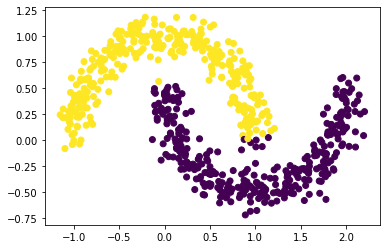
# plot a scatterplot to show the spectral clustering of data set with n = 1000 and noise = 0.1
plt.scatter(X[:, 0], X[:, 1], c = spectral_clustering(X, epsilon))
Based on the three graphs above, we found out that spectral clustering works well for different n, especially for smaller n. Also, as n increases, the points shown on the graphs around the two-half moon becomes larger, but the points try to gather together in each half moon.
Data Set Comparison: Same n But Different noise
# n = 600 and noise = 0.03
# set the size of the data set
n = 600
# control the randomness for each time running this cell
np.random.seed(1234)
# generate a date set of size n with data points forming as two
# moons and a data set of size n with integer labels of each moon
X, y = datasets.make_moons(n_samples = n, shuffle = True, noise = 0.03, random_state = None)
# plot a scatterplot to show the spectral clustering of data set with n = 600 and noise = 0.03
plt.scatter(X[:, 0], X[:, 1], c = spectral_clustering(X, epsilon))
# n = 600 and noise = 0.15
# set the size of the data set
n = 600
# control the randomness for each time running this cell
np.random.seed(1234)
# generate a date set of size n with data points forming as two
# moons and a data set of size n with integer labels of each moon
X, y = datasets.make_moons(n_samples = n, shuffle = True, noise = 0.15, random_state = None)
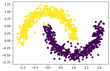
# plot a scatterplot to show the spectral clustering of data set with n = 600 and noise = 0.15
plt.scatter(X[:, 0], X[:, 1], c = spectral_clustering(X, epsilon))

# n = 600 and noise = 0.3
# set the size of the data set
n = 600
# control the randomness for each time running this cell
np.random.seed(1234)
# generate a date set of size n with data points forming as two
# moons and a data set of size n with integer labels of each moon
X, y = datasets.make_moons(n_samples = n, shuffle = True, noise = 0.3, random_state = None)
# plot a scatterplot to show the spectral clustering of data set with n = 600 and noise = 0.3
plt.scatter(X[:, 0], X[:, 1], c = spectral_clustering(X, epsilon))
Based on the three graphs above, we found out that spectral clustering has a lower ability to separate the data set as noise increases. This is because the points try to spread out from the center for each cluster and make the points in two clusters be very close, resulting the spectral clustering does not recognize which point is in which cluster.
Part I -- Does our spectral clustering work well for other data set?
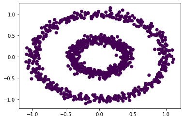
Now let's try our spectral clustering function on another data set -- the bull's eye!
# set the size of the data set
n = 1000
# generate a date set of size n with data points forming as two concentric
# circles and a data set of size n with integer labels of each moon
X, y = datasets.make_circles(n_samples=n, shuffle=True, noise=0.05, random_state=None, factor = 0.4)
# plot a scatterplot to show the data set
plt.scatter(X[:,0], X[:,1])
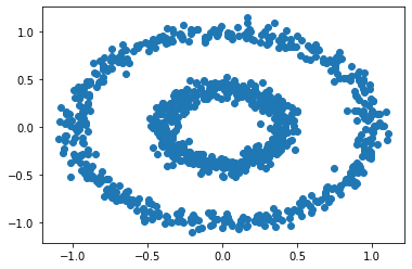
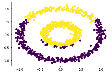
There are two concentric circles in the above graph. Let's try k-means for this data set.
# compute k-means clustering with two clusters
km = KMeans(n_clusters = 2)
# fit the data points in k-means
km.fit(X)
# plot a scatterplot based on the Euclidean coordinates of the
# data points with a group color, predicting by the k-means
plt.scatter(X[:,0], X[:,1], c = km.predict(X))
As before k-means does not do well here at all. But spectral clustering might do well here. Let's try for some values of epsilon for our function spectral_clustering(X, epsilon).
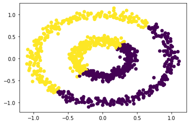
# plot a scatterplot to show the spectral clustering with epsilon = 0.22
plt.scatter(X[:, 0], X[:, 1], c = spectral_clustering(X, epsilon = 0.22))
# plot a scatterplot to show the spectral clustering with epsilon = 0.4
plt.scatter(X[:, 0], X[:, 1], c = spectral_clustering(X, epsilon = 0.4))
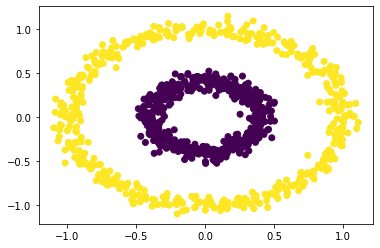
# plot a scatterplot to show the spectral clustering with epsilon = 0.54
plt.scatter(X[:, 0], X[:, 1], c = spectral_clustering(X, epsilon = 0.54))
Based on the above graphs, we may conclude that the spectral clustering will work when the epsilon is roughly between 0.22 and 0.54. Also, we may find out that spectral clustering will also work for data sets that look like two concentric circles.
Part J -- The end.
Great! That's all for our brief tutorial on spectral clustering.