Stancy Zhang

Goal

Diving into the intricate universe of linear modeling, this study handcrafts Ridge and Lasso regressions to shed light on their inner workings. By designing these models from scratch and meticulously contrasting their performance, we unravel the intricacies of their error landscapes, offering a comprehensive understanding of how each regression uniquely interprets data.

Import packages

import numpy as np
import matplotlib.pyplot as plt
import scipy.linalg as la
from time import time
import scipy.optimize as opt

Linear Models

A standard problem in statistics to solve the multivariate linear regression problem. \begin{equation} y = X * \beta + \epsilon \end{equation} The above notation is standard in statistics, but in our discussion (and codes) we will replace $\beta$ with b

y = X * b + eps.

X is known as the design matrix, and consists of n rows of observations, each of which has p features (so it is an $n\times p$ matrix). y is a vector of n responses. b is an unknown vector of p coefficients which we would like to find. eps (epsilon) is a vector of length n with random noise, typically i.i.d. normally distributed with variance sig (sigma).

In numpy notation, we could express this as

y[i] = np.dot(X[i], b) + sig * np.random.randn()

We want to determine b, so that when me make a new observation X[n] we can predict the response y[n]. One way to do this is to minimize the mean square error

\begin{equation} \mathop{\mathsf{minimize}}_b \mathbb{E}((X[n]*b - y[n])^2) \end{equation}

The solution to this is the solution to the least squares problem \begin{equation} \mathop{\mathsf{minimize}}_b \frac{1}{n} |X*b - y|_2^2 \end{equation}

Where $n$ is the number of rows in $X$. We'll let the solution to the problem be denoted $\hat{b}$, or bhat.

Generating Data

def gen_lstsq(n, p, sig=0.1):
    """
    Generate a linear least squares problem.
    
    Input
    ----------
    n: an integer represents number of rows of observations
    p: an integer represents number of features
    sig=0.1: a number represents variance decides random noise with default 0.1
    
    Output
    ----------
    X: nxp numpy matrix in random numbers
    y: nx1 numpy vector
    b: px1 numpy vector in random numbers
    """
    # generate nxp matrix X and px1 vector b
    X = np.random.randn(n, p)
    b = np.random.randn(p)
    # use the formula above: y = X * b + eps
    y = np.dot(X, b) + sig * np.random.randn(n)
    return X, y, b

QR factorization

If we form a QR factorization $X = QR$, we can find $\hat{b} = R^{-1} Q^T y$.

def solve_lstsq_qr(X, y):
    """
    Estimate b using the QR factorization.
    Codes are similar to the reader lecture notes,
    based on least squares solution ||y - X * b_hat||.
    
    Input
    ----------
    X: nxp numpy matrix in random numbers
    y: nx1 numpy vector
    
    Output
    ----------
    bhat: px1 numpy vector
    """
    # QR factorization
    Q, R = la.qr(X, mode='economic')
    # estimate b
    bhat = la.solve_triangular(R, Q.T @ y, lower=False)
    return bhat

Normal Equations

Often, this is the way statistics textbooks solve the problem: $\hat{b} = (X^T X)^{-1} X^T y$. This is based on the normal equation $X^T X \hat{b} = X^T y$.

def solve_lstsq_normal(X, y):
    """
    Estimate b using the normal equations, involving Cholesky factorization.
    
    Input
    ----------
    X: nxp numpy matrix in random numbers
    y: nx1 numpy vector
    
    Output
    ----------
    bhat: px1 numpy vector
    """
    # form Cholesky factorization
    L = np.linalg.cholesky(X.T @ X)
    # estimate b
    bhat = la.solve_triangular(L.T, 
                            la.solve_triangular(L, X.T @ y, lower=True),
                            lower=False)
    return bhat

Check the functions

We can generate a few random problems to test that solve_lstsq_qr and solve_lstsq_normal give the same prediction $\hat{b}$ (measure $|\hat{b}{qr} - \hat{b}{normal}|_2$ and check it is smaller than 1e-4). Check against solve_lstsq in numpy or scipy as well.

# first test
n = 300
p = 100
X, y, b = gen_lstsq(n, p, sig=0.1)
b_QR = solve_lstsq_qr(X, y)
b_normal = solve_lstsq_normal(X, y)
# measure the norm
la.norm(b_QR - b_normal) < 1e-4

True

# calculate solve_lstsq
b_scipy = la.lstsq(X, y)[0]
# measure the difference: QR estimation
la.norm(b_scipy - b_QR) < 1e-4

True

# measure the difference: normal estimation
la.norm(b_scipy - b_normal) < 1e-4

True

n = 300
p = 100
X, y, b = gen_lstsq(n, p, sig=0.1)
b_QR = solve_lstsq_qr(X, y)
b_normal = solve_lstsq_normal(X, y)
# measure the norm
la.norm(b_QR - b_normal) < 1e-4

True

# calculate solve_lstsq
b_scipy = la.lstsq(X, y)[0]
# measure the difference: QR estimation
la.norm(b_scipy - b_QR) < 1e-4

True

# measure the difference: normal estimation
la.norm(b_scipy - b_normal) < 1e-4

True

# second test
n = 150
p = 70
X, y, b = gen_lstsq(n, p, sig=0.1)
b_QR = solve_lstsq_qr(X, y)
b_normal = solve_lstsq_normal(X, y)
# measure the norm
la.norm(b_QR - b_normal) < 1e-4

True

# calculate solve_lstsq
b_scipy = la.lstsq(X, y)[0]
# measure the difference: QR estimation
la.norm(b_scipy - b_QR) < 1e-4

True

# measure the difference: normal estimation
la.norm(b_scipy - b_normal) < 1e-4

True

n = 150
p = 70
X, y, b = gen_lstsq(n, p, sig=0.1)
b_QR = solve_lstsq_qr(X, y)
b_normal = solve_lstsq_normal(X, y)
# measure the norm
la.norm(b_QR - b_normal) < 1e-4

True

# calculate solve_lstsq
b_scipy = la.lstsq(X, y)[0]
# measure the difference: QR estimation
la.norm(b_scipy - b_QR) < 1e-4

True

# measure the difference: normal estimation
la.norm(b_scipy - b_normal) < 1e-4

True

Estimate the Error

Estimate the error in the fit using the equation $\frac{1}{n}|X * \hat{b} - y|_2^2$.

def err(X, y, bhat):
    """
    Estimate the error by using (1/n) ||X * bhat - y||^2
    
    Input
    ----------
    X: nxp numpy matrix in random numbers
    y: nx1 numpy vector
    bhat: px1 numpy vector
    
    Output
    ----------
    error: a number represents error in the fit
    """
    # get n by length of y
    n = len(y)
    # calculate error
    error = (1/n) * np.power(la.norm(X @ bhat - y), 2)
    return error

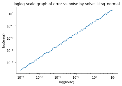
# plot error vs noise parameter sig
n = 100
p = 50
# sig in logarithmic distribution
sig = np.power(10, np.linspace(-4, 1, n+1))

error = []
for s in sig:
    # generate X, y, and bhat
    X, y, b = gen_lstsq(n, p, s)
    bhat = solve_lstsq_normal(X, y)
    error.append(err(X, y, bhat))
plt.loglog(sig, error)
plt.xlabel("log(noise)")
plt.ylabel("log(error)")
plt.title("loglog-scale graph of error vs noise by solve_lstsq_normal")

Text(0.5, 1.0, 'loglog-scale graph of error vs noise by solve_lstsq_normal')

png

Which of `solve_lstsq_qr` and `solve_lstsq_normal` is faster?

n = 100
p = 50
X, y, b = gen_lstsq(n, p, sig=0.1)
start = time()
b_QR = solve_lstsq_qr(X, y)
end = time()
print("Time of solve_lstsq_qr is " + str(end-start) + "s.")

Time of solve_lstsq_qr is 0.006086111068725586s.

start = time()
b_normal = solve_lstsq_normal(X, y)
end = time()
print("Time of solve_lstsq_normal is " + str(end-start) + "s.")

Time of solve_lstsq_normal is 0.0029091835021972656s.

Based on the time above that 0.006086111068725586s (solve_lstsq_qr) > 0.0029091835021972656s (solve_lstsq_normal), solve_lstsq_normal is slightly faster.

Number of operations of solve_lstsq_qr:$\frac{2n^3}{3}$
Number of operations of solve_lstsq_normal: $\frac{n^3}{3}$

Asymptotically, both of them order are ${O(p^3)}$.

Optimization Question

Solve the minimization problem \begin{equation} \mathop{\mathsf{minimize}}_b \frac{1}{n}|X*b - y|_2^2 \end{equation}

We'd like to minimize the objective function \begin{equation} n f(b) = |X*b - y|_2^2 = (Xb - y)^T (Xb - y) = b^T X^T X b - 2 y^T X b + y^T y \end{equation}

We might write the above expression as \begin{equation} n f(b) \sum_{i,j} b_i (X^T X){i,j} b_j - 2\sum{j,i} y_i X_{i,j} b_j + y^T y \end{equation}

We can take a derivative with respect to $b_j$ \begin{equation} n \frac{\partial f}{\partial b_j} = \sum_{i\ne j} b_i (X^T X){i,j} + \sum{i\ne j} (X^T X){j,i} b_i + 2 (X^T X){j,j} b_j - 2\sum_{i} y_i X_{i,j} \end{equation}

Putting this in matrix form, we obtain \begin{equation} J_f(b) = \frac{1}{n}\big( b^T (X^T X) + b^T (X^T X)^T - 2y^T X\big) = \frac{2}{n} b^T (X^T X) -\frac{2}{n}y^T X \end{equation}

So we can write $J_f(b) = \frac{2}{n} b^T (X^T X) -\frac{2}{n} y^T X$

def solve_lstsq_opt(X, y):
    """
    Solve the minization problem.
    
    Input
    ----------
    X: nxp numpy matrix in random numbers
    y: nx1 numpy vector
    
    Output
    ----------
    solver: a number represents the minization solution
    """
    n, p = X.shape
    # define the objective function
    def f(b):
        """
        Define function: (1/n)||X * b - y||^2
        
        Input
        ----------
        b: px1 numpy vector

        Output
        ----------
        f_b: a number represents the function value
        """
        f_b = (1/n) * np.power(la.norm(X @ b - y), 2)
        return f_b
    # define Jacobian
    def Jf(b):
        """
        Find the Jacobian of the function
        
        Input
        ----------
        b: px1 numpy vector

        Output
        ----------
        Jf_b: a vector represents the Jacobian of the function
        """
        Jf_b = (2/n) * b.T @ (X.T @ X) - (2/n) * y.T @ X
        return Jf_b
    solver = opt.minimize(f, np.random.rand(p), jac = Jf)
    return solver

Check

We can generate a few random problems to test that solve_lstsq_opt agrees with solve_lstsq_qr and solve_lstsq_normal.

# first test
n = 300
p = 100
X, y, b = gen_lstsq(n, p, sig=0.1)
b_QR = solve_lstsq_qr(X, y)
b_normal = solve_lstsq_normal(X, y)
# x is the solution array
b_opt = solve_lstsq_opt(X, y).x

# measure the difference: QR estimation
la.norm(b_opt - b_QR) < 1e-4

True

# measure the difference: normal estimation
la.norm(b_opt - b_normal) < 1e-4

True

n = 300
p = 100
X, y, b = gen_lstsq(n, p, sig=0.1)
b_QR = solve_lstsq_qr(X, y)
b_normal = solve_lstsq_normal(X, y)
# x is the solution array
b_opt = solve_lstsq_opt(X, y).x

# measure the difference: QR estimation
la.norm(b_opt - b_QR) < 1e-4

True

# measure the difference: normal estimation
la.norm(b_opt - b_normal) < 1e-4

True

# second test
n = 150
p = 70
X, y, b = gen_lstsq(n, p, sig=0.1)
b_QR = solve_lstsq_qr(X, y)
b_normal = solve_lstsq_normal(X, y)
# x is the solution array
b_opt = solve_lstsq_opt(X, y).x

# measure the difference: QR estimation
la.norm(b_opt - b_QR) < 1e-4

True

# measure the difference: normal estimation
la.norm(b_opt - b_normal) < 1e-4

True

n = 150
p = 70
X, y, b = gen_lstsq(n, p, sig=0.1)
b_QR = solve_lstsq_qr(X, y)
b_normal = solve_lstsq_normal(X, y)
# x is the solution array
b_opt = solve_lstsq_opt(X, y).x

# measure the difference: QR estimation
la.norm(b_opt - b_QR) < 1e-4

True

# measure the difference: normal estimation
la.norm(b_opt - b_normal) < 1e-4

True

How fast is `solve_lstsq_opt` compared to the functions above?

n = 300
p = 100
X, y, b = gen_lstsq(n, p, sig=0.1)
start = time()
b_opt = solve_lstsq_opt(X, y)
end = time()
print("Time of solve_lstsq_opt(X, y) is " + str(end-start) + "s.")

Time of solve_lstsq_opt(X, y) is 0.051744937896728516s.

# number of evaluations of the objective functions
b_opt.nfev

0.051744937896728516s (solve_lstsq_opt) > 0.006086111068725586s (solve_lstsq_qr) > 0.0029091835021972656s (solve_lstsq_normal)

Comparing to the functions in Part A, solve_lstsq_opt is much slower.

Comparing ${O(p^2 * n * nfev)}$ (solve_lstsq_opt) and ${O(p^3)}$ (solve_lstsq_qr and solve_lstsq_normal),

${O(p^2 * n * nfev)}$ is much larger mainly because of ${nfev}$ which is large. (we can consider ${O(p^2 * n)}$ and ${O(p^3)}$ are basically the same asymptotically)

Ridge Regression

We'll now turn to the problem of what to do when n < p. In this case we can find a $b$ which satisfies the equation $X * b = y$ exactly, but there are many possible values of $b$ which can satisfy the equation.

Ridge regression seeks to solve the following optimization problem:

\begin{equation} \mathop{\mathsf{minimize}}_b \frac{1}{n}|X*b - y|_2^2 + \lambda |b|_2^2 \end{equation}

$\lambda$ is the regularize parameter.

Optimization

Jacobian for the objective function for the minimization problem is below, by linearity,

$J_f(b) = \frac{2}{n} b^T (X^T X) -\frac{2}{n} y^T X + 2\lambda b$

def solve_ridge_opt(X, y, lam=0.1):
    """
    Solve the minization problem.
    
    Input
    ----------
    X: nxp numpy matrix in random numbers
    y: nx1 numpy vector
    lam: a number represents the regularization term
    
    Output
    ----------
    solver: a number represents the minization solution
    """
    n, p = X.shape
    # define the objective function
    def f(b):
        """
        Define function: (1/n)||X * b - y||^2 + lam ||b||^2
        
        Input
        ----------
        b: px1 numpy vector

        Output
        ----------
        f_b: a number represents the function value
        """
        f_b = (1/n) * np.power(la.norm(X @ b - y), 2) + lam * np.power(la.norm(b), 2)
        return f_b
    # define Jacobian
    def Jf(b):
        """
        Find the Jacobian of the function
        
        Input
        ----------
        b: px1 numpy vector

        Output
        ----------
        Jf_b: a vector represents the Jacobian of the function
        """
        Jf_b = (2/n) * b.T @ (X.T @ X) - (2/n) * y.T @ X + 2 * lam * b
        return Jf_b
    solver = opt.minimize(f, np.random.rand(p), jac = Jf)
    return solver

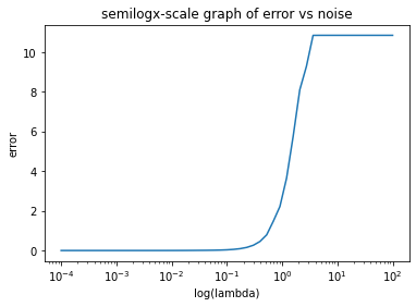
Compute the error

Set n = 50, p=100, and sig=0.1. Let's make a plot that displays the error of bhat computed using solve_ridge_opt as lam varies between 1e-4 and 1e2.

# plot error vs lambda
n = 50
p = 100
sig = 0.1
X, y, b = gen_lstsq(n, p, sig)
# lam in logarithmic distribution
lam = np.power(10, np.linspace(-4, 2, n+1))

error = []
for l in lam:
    # generate X and y
    bhat = solve_ridge_opt(X, y, l).x
    error.append(err(X, y, bhat))
plt.semilogx(lam, error)
plt.xlabel("log(lambda)")
plt.ylabel("error")
plt.title("semilogx-scale graph of error vs noise")

Text(0.5, 1.0, 'semilogx-scale graph of error vs noise')

png

Lasso

The Lasso is L1-regularized regression. This is often used when p > n, and when the parameter vector b is assumed to be sparse, meaning that it has few non-zero entries.

The minimization problem is \begin{equation} \mathop{\mathsf{minimize}}_b \frac{1}{n} |X * b - y|_2^2 + \lambda |b|_1 \end{equation}

Where again, $\lambda$ can be chosen.

Generate Data

We need to modify our generation of data to produce sparse b.

def gen_lstsq_sparse(n, p, sig=0.1, k=10):
    """
    Generate a linear least squares problem.
    
    Input
    ----------
    n: an integer represents number of rows of observations
    p: an integer represents number of features
    sig=0.1: a number represents variance decides random noise with default 0.1
    k=10: an integer represents the number of random entries that set to 1 with default 10
    
    Output
    ----------
    X: nxp numpy matrix in random numbers
    y: nx1 numpy vector
    b: px1 numpy vector in random numbers
    """
    # generate nxp matrix X and px1 vector b
    X = np.random.randn(n, p)
    b = np.zeros(p)
    # get k random enrties that will be set to 1
    non_zero_pos = np.random.choice(p,k)
    for i in non_zero_pos:
        b[i] = 1
    
    # use the formula above: y = X * b + eps
    y = np.dot(X, b) + sig * np.random.randn(n)
    return X, y, b

Optimization

Recall we want to find bhat to solve \begin{equation} \mathop{\mathsf{minimize}}_b \frac{1}{n} |X * b - y|_2^2 + \lambda |b|_1 \end{equation}

Jacobian for the objective function for the minimization problem is below,

$J_f(b) = \frac{2}{n} b^T (X^T X) -\frac{2}{n} y^T X + \lambda sign(b)$

note that np.sign(0) = 0

def solve_lasso_opt(X, y, lam=0.1):
    """
    Solve the minization problem.
    
    Input
    ----------
    X: nxp numpy matrix in random numbers
    y: nx1 numpy vector
    lam: a number represents the regularization term
    
    Output
    ----------
    solver: a number represents the minization solution
    """
    n, p = X.shape
    # define the objective function
    def f(b):
        """
        Define function: (1/n)||X * b - y||(2)^2 + lam ||b||(1)
        
        Input
        ----------
        b: px1 numpy vector

        Output
        ----------
        f_b: a number represents the function value
        """
        f_b = (1/n) * np.power(la.norm(X @ b - y), 2) + lam * la.norm(b, 1)
        return f_b
    # define Jacobian
    def Jf(b):
        """
        Find the Jacobian of the function
        
        Input
        ----------
        b: px1 numpy vector

        Output
        ----------
        Jf_b: a vector represents the Jacobian of the function
        """
        Jf_b = (2/n) * b.T @ (X.T @ X) - (2/n) * y.T @ X + lam * np.sign(b)
        return Jf_b
    solver = opt.minimize(f, np.random.rand(p), jac = Jf)
    return solver

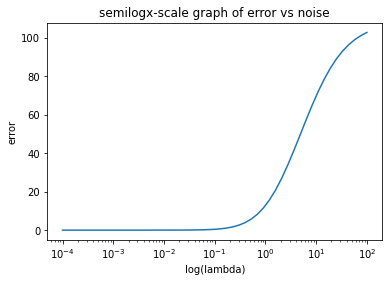
Compute the Error

Set n = 50, p=100,sig=0.1, and k=10 to generate a problem using gen_lstsq_sparse.

# plot error vs lambda
n = 50
p = 100
sig = 0.1
k = 10
X, y, b = gen_lstsq_sparse(n, p, sig, k)
# lam in logarithmic distribution
lam = np.power(10, np.linspace(-4, 2, n+1))

error = []
for l in lam:
    # generate X and y
    bhat = solve_lasso_opt(X, y, l).x
    error.append(err(X, y, bhat))
# print(bhat)
plt.semilogx(lam, error)
plt.xlabel("log(lambda)")
plt.ylabel("error")
plt.title("semilogx-scale graph of error vs noise")

Text(0.5, 1.0, 'semilogx-scale graph of error vs noise')

png

Goal

Import packages

Linear Models

Generating Data

QR factorization

Normal Equations

Check the functions

Estimate the Error

Which of solve_lstsq_qr and solve_lstsq_normal is faster?

Optimization Question

Check

How fast is solve_lstsq_opt compared to the functions above?

Ridge Regression

Optimization

Compute the error

Lasso

Generate Data

Optimization

Compute the Error

Which of `solve_lstsq_qr` and `solve_lstsq_normal` is faster?

How fast is `solve_lstsq_opt` compared to the functions above?